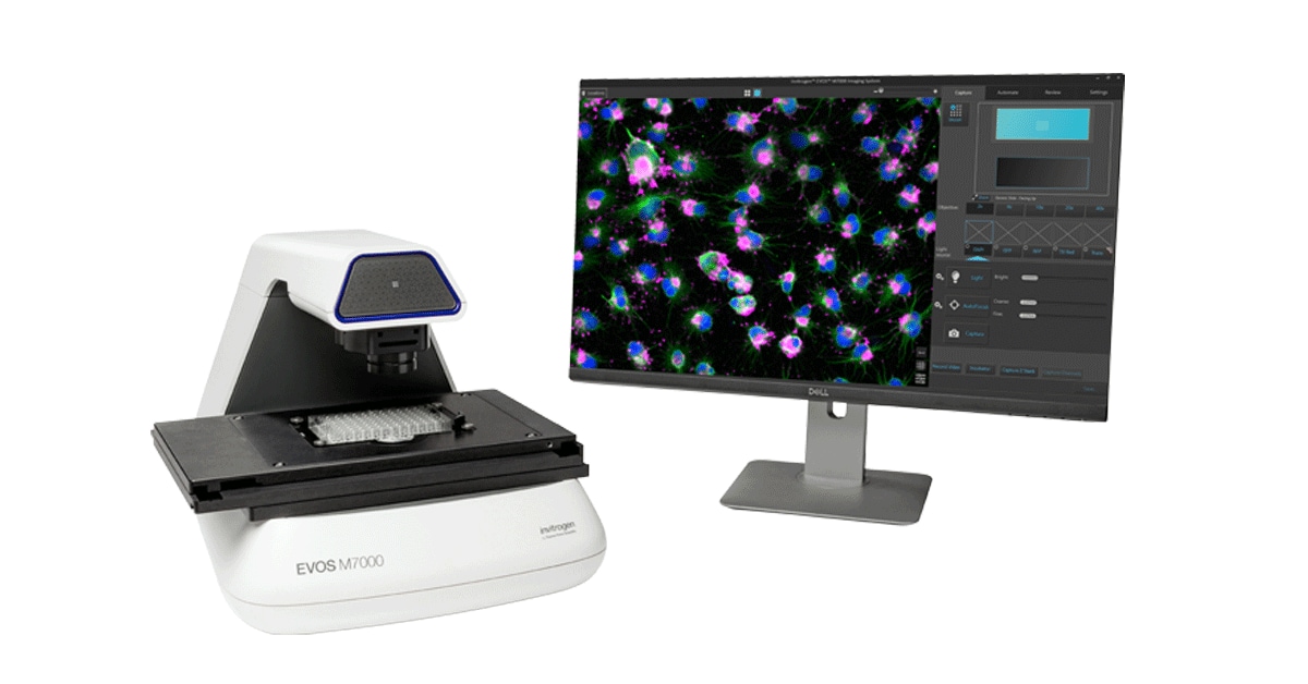
🎬 Watch: Z-Stacking & 3D Analysis in Action
See EVOS M7000 capture multi-layer images and reconstruct 3D models — from Thermo Fisher
What is Z-Stacking?
Z-stacking (also called optical sectioning) captures a series of images at different focal depths through a thick sample. Instead of one blurry 2D image, you get a stack of sharp images representing different "slices" through your cells.
Why Standard 2D Imaging Falls Short
- Thick samples: A cell monolayer might be 10μm, but organoids and tissue sections are 100-500μm thick
- Out-of-focus blur: In a single image, only one plane is sharp; everything above and below is blurry
- 3D structures lost: Spheroids, neurons, and tissue architecture can't be understood from one slice
- Quantification errors: Counting cells in 2D misses cells above/below the focal plane
How Z-Stacking Works
- Set Z range: Define top and bottom of your sample (e.g., 0μm to 200μm)
- Set step size: Typically 2-10μm between slices depending on objective NA
- Auto-capture: System moves focus motor and captures at each Z position
- Result: 20-100 individual images forming a 3D dataset
Example: A 200μm organoid with 5μm steps = 40 images in the Z-stack
2D Deconvolution: Sharpening Every Slice
Even within each Z-slice, there's some out-of-focus light from above and below. Deconvolution mathematically removes this blur.
How Deconvolution Works
- Point Spread Function (PSF): Characterizes how a perfect point of light blurs in your optical system
- Mathematical reversal: Algorithm "un-blurs" each pixel based on the PSF
- Iterative refinement: Richardson-Lucy algorithm runs 10-50 iterations to converge on sharp image
- Result: Higher contrast, better signal-to-noise, crisper subcellular detail
🔬 Deconvolution vs No Deconvolution
| Feature | Raw Image | Deconvolved |
|---|---|---|
| Nuclear boundary | Fuzzy edge | Sharp, crisp edge |
| Mitochondria detail | Blurred rods | Individual organelles visible |
| Signal-to-noise | Low (hazy background) | High (clean signal) |
| Quantification | ±20% error | ±5% error |
Why 2D Deconvolution is Important
Even if you're not doing 3D analysis, 2D deconvolution alone transforms image quality. Here's why it matters for every fluorescence microscopist:
The Problem: Out-of-Focus Haze
Every fluorescence image contains out-of-focus light — photons from above and below the focal plane that blur into your image. This reduces contrast and makes fine structures disappear.
- Signal-to-noise drops: Haze adds background that drowns out weak signals
- Resolution appears worse: Two nearby objects merge into one blob
- Quantification suffers: Fluorescence intensity measurements are inflated by background haze
- Subcellular detail lost: Mitochondria, vesicles, and filaments become indistinct
What Deconvolution Does
Deconvolution mathematically re-assigns out-of-focus photons back to their origin. It's like "focusing" the image after capture using knowledge of your optical system.
- Higher contrast: Background haze reduced by 60-80%
- Sharper edges: Nuclear and cell boundaries become crisp
- Better resolution: Structures 20-30% closer together become distinguishable
- Accurate intensity: Fluorescence quantification reflects true signal, not background
- Noise handling: Advanced algorithms (Richardson-Lucy with regularization) separate signal from noise
⚠️ Common Misconception
Deconvolution does NOT create data that isn't there. It re-assigns photons that ARE in your image to their correct locations. If two structures are closer than the Abbe limit (~200nm for visible light), deconvolution cannot separate them — but it CAN make them appear sharper and more distinct at the limit.
Deconvolution vs Confocal Microscopy
Confocal microscopy is often seen as the "gold standard" for sharp optical sections. But deconvolution on widefield systems offers distinct advantages:
| Feature | Widefield + Deconvolution | Confocal (LSCM) |
|---|---|---|
| Light dose | ✅ Low — uses all available light | ❌ High — discards 90-95% of light through pinhole |
| Phototoxicity | ✅ Low — gentle on live cells | ❌ Higher — intense laser excitation damages cells over time |
| Speed | ✅ Fast — capture entire field at once | ❌ Slow — raster scan point-by-point |
| Cost | ✅ Affordable — standard fluorescence microscope | ❌ Expensive — £100K+ for laser scanning system |
| Live cell imaging | ✅ Excellent — low light, fast capture | ⚠️ Moderate — photobleaching limits duration |
| Thick samples (>50μm) | ⚠️ Moderate — scattering limits penetration | ✅ Excellent — optical sectioning rejects scatter |
| Resolution | ✅ Good — near-diffraction limited after deconvolution | ✅ Slightly better — ~1.4x improvement in XY |
| 3D reconstruction | ✅ Excellent — computational sectioning is sharp | ✅ Excellent — physical optical sectioning |
| Signal-to-noise | ✅ Better for dim samples — collects more photons | ⚠️ Worse for dim samples — pinhole rejects most signal |
When to Choose Deconvolution Over Confocal
- Live cell imaging: Low phototoxicity lets you image for hours/days without killing cells
- Dim fluorescent samples: Weak signals that would be lost through a confocal pinhole
- High-throughput screening: Fast capture of multi-well plates (confocal too slow)
- Budget constraints: £10K widefield + deconvolution vs £150K confocal
- Quantitative fluorescence: More photons = better intensity measurements
- Cell monolayers (<20μm): Widefield + deconvolution is often sharper than confocal at same thickness
When Confocal Wins
- Thick tissue sections (>50μm): Scattering makes widefield unusable; confocal rejects out-of-focus scatter
- Very dense samples: When fluorescence from neighboring cells overwhelms deconvolution
- Super-resolution needs: STED or Airyscan confocal beats deconvolution for sub-200nm structures
- Simultaneous multicolor: Some confocals have better spectral separation for 4+ channels
💡 The EVOS M7000 Advantage
The EVOS M7000 combines widefield speed and sensitivity with real-time deconvolution — giving you confocal-like sectioning without the cost, speed penalty, or phototoxicity. For cell culture labs doing 2D monolayers, spheroids up to 200μm, and live cell time-lapse, it's often the better choice than a £100K+ confocal system.
3D Visualization: Seeing the Full Picture
Once you have a deconvolved Z-stack, software can reconstruct the 3D structure:
Visualization Modes
- Maximum Intensity Projection (MIP): brightest pixel through the stack displayed as 2D — great for overview
- Volume rendering: Full 3D model with transparency, rotation, clipping planes
- Orthogonal views: XY, XZ, and YZ planes shown simultaneously for precise localization
- Surface rendering: 3D mesh models of cell boundaries for morphometric analysis
EVOS M7000 3D Analysis Features
- Automated Z-stack capture: Set range and step, system does the rest
- Real-time deconvolution: Process while capturing, no waiting
- 3D cell counting: Count objects through entire volume, not just one plane
- Volume measurement: Calculate spheroid/organoid volume in μm³
- Colocalization analysis: See if two proteins interact in 3D space
- Export: TIFF stacks, AVI movies, 3D models for publications
Applications of Z-Stacking in Cell Culture
| Application | Z-Stack Benefit | Why It Matters |
|---|---|---|
| Tumor spheroid screening | Volume measurement | Drug efficacy better predicted by 3D volume than 2D area |
| Neurite outgrowth | 3D tracing | Measure total neurite length in 3D, not just 2D projection |
| Stem cell colonies | Layer analysis | Detect stratification and differentiation markers at different depths |
| Immunofluorescence | Colocalization | Verify protein-protein interaction in true 3D space |
| Tissue sections | Full thickness imaging | See entire 50μm section without missing surface or deep layers |
| Organ-on-chip | Lumen measurement | Measure hollow organoid lumen diameter in 3D |
💡 Pro Tips for Z-Stacking
- Step size rule: Use ~0.5 × optical slice thickness (e.g., 2μm steps for 4μm slice with 20x/0.45 NA)
- Nyquist sampling: Sample at least twice per axial resolution unit to avoid missing structures
- Over-sample then project: It's better to capture too many slices and project down than miss a layer
- Use deconvolution: Always deconvolve before 3D analysis — it improves every downstream measurement
- Start focus high: Begin above your sample and focus down to ensure you capture the top
🎬 Watch the Full Video
See EVOS M7000 Z-stacking and 3D analysis in action:
▶ Watch on YouTubeRead EVOS M3000 Review →